MEP

Molecular Electrostatic Potential (MEP)

The molecular electrostatic potential (MEP) at a given point p(x,y,z) in the vicinity of a molecule is the force acting on a positive test charge (a proton) located at p through the electrical charge cloud generated through the molecules electrons and nuclei. Despite the fact that the molecular charge distribution remains unperturbed through the external test charge (no polarization occurs) the electrostatic potential of a molecule is still a good guide in assessing the molecules reactivity towards positively or negatively charged reactants. The MEP is typically visualized through mapping its values onto the surface reflecting the molecules boundaries. The latter can be generated through overlapping the vdW radii of all atoms of the molecule, through algorithms calculating the solvent accessible surface of the molecule, or through a constant value of electron density. The latter will be used here to answer the question of which site in imidazole is particularly attractive to a proton. Imidazole contains two nitrogen atoms both of which might act as proton acceptor sites.

In order to calculate the MEP of imidazole we first optimize the geometry of the system at the Becke3LYP/6-31G(d) level of theory. Visualization of the MEP then requires three more steps:

1) Calculation of the outer envelope of imidazole as defined through a constant value of electron density.

2) Calculation of the MEP at a number of points around the molecule.

3) Mapping of the MEP on the molecular surface using a color coded scheme.

Calculation of the outer envelope of imidazole can be achieved using the following input file:

#P Becke3LYP/6-31G(d) cube=(medium,density) scf=tight

Becke3LYP/6-31G(d) imidazole density

0 1
C,0,-0.9741771331,0.,-0.6301926171
C,0,-0.907244165,0.,0.7404218415
N,0,0.4034833469,0.,1.1675913068
C,0,1.124080815,0.,0.0676366081
N,0,0.3402990549,0.,-1.0525852362
H,0,0.6597356899,0.,-2.0102490569
H,0,-1.8002953135,0.,-1.3251503429
H,0,-1.7267332321,0.,1.4464261172
H,0,2.2048589411,0.,0.0167357941

imi_den.cub

In this particular example the density is calculated at a number of grid points around the molecule forming a three dimensional grid. The density of points per direction is specified as "medium" in this particular example (equal to 80 points per direction and 512000 points in total). The results are stored in the file "imi_den.cub".

In a second run the MEP is calculated in a similar way again on a number of grid points and stored in another file "imi_pot.cub".


#P Becke3LYP/6-31G(d) int=finegrid scf=tight
 geom=check guess=read cube=(medium,potential)

Becke3LYP/6-31G(d) imidazole potential

0 1

imi_pot.cub

More recent versions of Gaussian do not fully support the cube keyword anymore. It is then advisable to generate the cubes separately from the formatted checkpoint file using the cubegen utility program. How this can be combined with generation of the formatted checkpoint file is shown below for the example of imidazole at the Becke3LYP/6-31G(d) level using the following PBS job script named "imi1":

#!/bin/csh
#PBS -l mem=128mb
#PBS -q long
setenv g03root /usr/local
setenv GAUSS_SCRDIR /scratch
setenv GAUSS_EXEDIR /usr/local/g03b3
setenv GAUSS_ARCHDIR /usr/local/g03b3
setenv LD_LIBRARY_PATH "${GAUSS_EXEDIR}:/usr/lib"
cat >$GAUSS_SCRDIR/$PBS_JOBNAME << EOF
%chk=/scratch/imi1.chk
%mem=6000000
#P Becke3LYP/6-31G(d) scf=tight formcheck

Becke3LYP/6-31G(d) imidazole density + ESP

0 1
C,0,-0.9741771331,0.,-0.6301926171
C,0,-0.907244165,0.,0.7404218415
N,0,0.4034833469,0.,1.1675913068
C,0,1.124080815,0.,0.0676366081
N,0,0.3402990549,0.,-1.0525852362
H,0,0.6597356899,0.,-2.0102490569
H,0,-1.8002953135,0.,-1.3251503429
H,0,-1.7267332321,0.,1.4464261172
H,0,2.2048589411,0.,0.0167357941


EOF
touch $PBS_O_WORKDIR/$PBS_JOBNAME.$HOST
/usr/local/g03b3/g03 < $GAUSS_SCRDIR/$PBS_JOBNAME > $GAUSS_SCRDIR/$PBS_JOBNAME.log
mv $GAUSS_SCRDIR/$PBS_JOBNAME.log $PBS_O_WORKDIR/$PBS_JOBNAME.log
mv $GAUSS_SCRDIR/$PBS_JOBNAME.chk $PBS_O_WORKDIR/$PBS_JOBNAME.chk
rm -f $GAUSS_SCRDIR/$PBS_JOBNAME
mv Test.FChk  $PBS_O_WORKDIR/$PBS_JOBNAME.fch
$GAUSS_EXEDIR/cubegen 0 Density=SCF $PBS_O_WORKDIR/$PBS_JOBNAME.fch $PBS_O_WORKDIR/$PBS_JOBNAME.den.cub 0 h
$GAUSS_EXEDIR/cubegen 0 Potential=SCF $PBS_O_WORKDIR/$PBS_JOBNAME.fch $PBS_O_WORKDIR/$PBS_JOBNAME.esp.cub 0 h
exit

What the additional lines after execution of Gaussian do is move the Gaussian output files from /scratch to the users working directory, move the formatted checkpoint file named "Test.FChk" to a more meaningful name (here: imi1.fch), and then call cubegen to first generate the cube file for the total electron density and then generate a cube file for the ESP. The program cubegen accepts six arguments on the command line. The first argument (here: 0) defines the memory allocated to the run. Using the argument of 0 specifies automatic memory allocation. The second argument defines the type of cube plot desired in this run. The particular argument here (Density=SCF) defines the total electron density as calculated at the SCF level. The third argument defines the name of the formatted checkpoint file, the fourth argument the name of the cube file, the fifth argument the number of points per side of the cube. Using the argument of -3 at this point leads to selection of a medium sized grid with 6 points/Bohr resolution. Finer grids can be selected with the argument -4, a coarser grid with the argument -2. Finally, the last argument indicates, whether a header (h) is to be included in the cube file. If this is not desired, the last argument must be n.
The above job script assumes that the name of the script itself is "imi1". For other names to work, the name of the checkpoint file must be altered.

Mapping of the MEP onto the molecular surface can be performed with GaussView in the following way. After starting GaussView load the cube file containing the density grid "imi1.den.cub". Don't forget to select the appropriate file type ".cub". After loading the file, select the "Surfaces..." option from the "Results" menu. The only surfaces available at that point are those defined through a constant value of total electron density. Which value is appropriate for the system at hand should be tested at that stage. Once a value has been chosen, the "Okay" button starts generation of the surface, which will appear in a new window.
In order to map the MEP onto this surface first load the second cube file containing the MEP data with the "Load..." button. After Loading has completed, reselect the density surface and choose "Map values from a 2nd surface". The colour coding of the MEP map can be adjusted in the new window that appears with the MEP map.

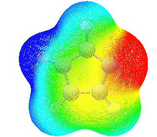
In this particular case the colours have been chosen such that regions of attractive potential appear in red and those of repulsive potential appear in blue. The resulting overall MEP of imidazole leaves no doubt that the nitrogen atom carrying a proton already (N5) is not attractive to a positive test charge while the opposite is true for N3. The MEP mapping can be further manipulated by selecting surfaces of different degree of transparency (under "View" - "Display Format.." - "Surface") as well as selecting new limits for the colour coding spectrum.

Detailed instructions for visualizing the MEP can also be found on the Gaussian home page.

last changes: 01.04.2008, AS
questions & comments to: axel.schulz@uni-rostock.de