Contracted Gaussian type orbitals

Minimal basis sets

---

            Single Gaussian functions as described by equ. (5) are not well suited to describe the spatial extend and nodal characteristics of atomic orbitals. To solve this problem, basis functions are described as a sum (a "contraction") of several Gaussian functions (primitives):

 

 

 

We will use the STO-3G basis set¹ for carbon as an example (here in a format produced by Gaussian 94):

 

C 0

 S    3 1.00

   .7161683735D+02   .1543289673D+00

   .1304509632D+02   .5353281423D+00

   .3530512160D+01   .4446345422D+00

 SP   3 1.00

   .2941249355D+01  -.9996722919D-01   .1559162750D+00

   .6834830964D+00   .3995128261D+00   .6076837186D+00

   .2222899159D+00   .7001154689D+00   .3919573931D+00

 

The format used is:

Shell_type,  No. of primitive Gaussians x,   Scale_factor

Orbital exponent a_x, Contraction coefficient d_x

(repeat x times)

 

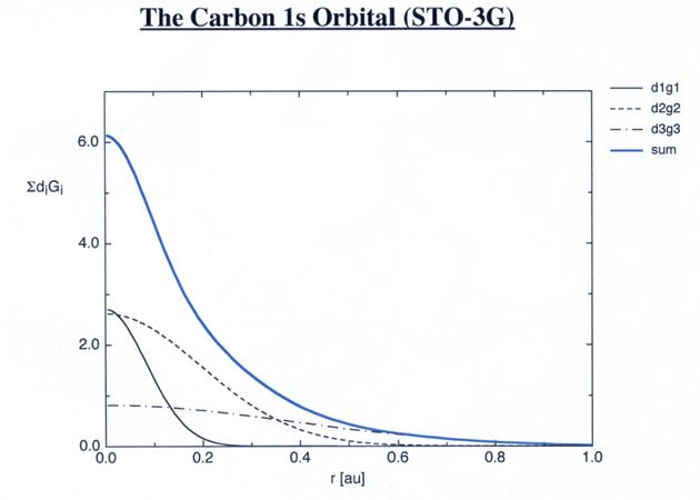
The first line specifies that the carbon 1s orbital will be described as a sum of three Gaussian primitives with different exponents a_1s,x and coefficients d_1s,x. The following three lines contain the exponent a_1s,x and coefficient d_1s,x for x=1, 2, and 3. Written in an explicit manner, the 1s basis function for carbon then equates to:

 

 

The basis sets for the 2s and 2p orbitals are also composed of a contraction of three Gaussian primitives and are specified together in one single "SP"-block. For the sake of computational efficiency, the 2s and 2p orbitals share the same exponents  a_2,x , but have different contraction coefficients. Each line of the basis set description therefore contains only one exponent (a_2s,x = a_2p,x ), but two different coefficients d_2s,x and d_2p,x. The nodal characteristics of the 2s-orbital are simulated using one coefficient with negative sign (-0.09996722919) and two coefficients with positive (+0.3995128261 and +0.7001154689) sign. Orbital exponents and coefficients have been optimized first for atomic calculations minimizing the energy of single atoms. Additional scale factors have, however, then been developed for use of these atomic basis functions in studies of small organic molecules. The STO-3G basis set thus contains an appreciable amount of "semiempirical" character!

 

            How many basis functions do we need for a small organic molecule such as methanol (CH₄O)?

 

%Kjob L301 #P HF/sto-3g GFInput GFPrint methanol basis set 0,1 C1 O2 1 r2 H3 1 r3 2 a3 H4 1 r4 2 a4 3 d4 r2=1.20 r3=1.0 r4=1.0 a3=120. a4=120. d4=180.

Kjob command kills the job after checking the input The GFInput (“Gaussian Function Input”) output generation keyword causes the current basis set to be printed in a form suitable for use as general basis set input, and can thus be used in adding to or modifying standard basis sets. GFPrint command: This output generation keyword prints the current basis set in tabular form.

 

 

For each of the atomic 1s, 2s and 2p-orbitals, the STO-3G basis set uses a contraction of three Gaussians. We thus have 5 basis functions for each carbon and oxygen atom, and only one basis function for each hydrogen, yielding a total of 14 basis functions (and 14 MO-coefficients to vary in the SCF calculations). Each of these basis functions consists of three Gaussian primitives, and the number of primitives is therefore 3*14=42. In the output file of Gaussian 98 the number of basis functions and primitives is given by link 301 together with the number of electrons and the core-core repulsion energy:

 

    14 basis functions       42 primitive gaussians

     9 alpha electrons        9 beta electrons

    nuclear repulsion energy        40.7431450799 Hartrees.

 

            How "good" is the STO-3G basis set? The answer to this question depends on the chemical problem at hand. Structural features of ground state molecules are reproduced quite often with surprisingly good accuracy at the HF/STO-3G level of theory. Table 1 lists structural parameters of methanol as predicted by a variety of theoretical methods.

 

Table 1. Structural features of methanol (C_s) as predicted by several theoretical methods.

 

HF/STO-3G                             1.432999                   103.856                  14

HF/3-21G                                 1.440922                   110.336                  26

HF/3-21+G                               1.454241                   113.291                  34

HF/6-31G                                 1.430503                   113.410                  26

HF/D95                                    1.437049                   113.874                  28

HF/6-31G(d)                            1.399562                   109.448                  38

HF/6-31G(d,p)                         1.398520                   109.650                  50

HF/6-31++G(d,p)                     1.401386                   110.542                  62

HF/6-311G(d,p)                       1.399240                   109.355                  60

HF/6-311++G(d,p)                   1.400243                   110.017                  72

HF/6-311G(2df,2pd)                1.396113                   109.836                  116

HF/cc-pVDZ                            1.397818                   109.116                  48

HF/cc-pVTZ                             1.398133                   109.937                  116

exp.                                           1.421                         108.0

last changes: 01.04.2008, AS
questions & comments to: axel.schulz@uni-rostock.de