The Polarizable Continuum Model (PCM)
The Polarizable Continuum Model (PCM) by Tomasi
and coworkers is one of the most frequently used continuum solvation methods
and has seen numerous variations over the years. The PCM model calculates the
molecular free energy in solution as the sum over three terms:
Gsol = Ges + Gdr + Gcav (1)
These components represent the electrostatic (es) and the dispersion-repulsion
(dr) contributions to the free energy, and the cavitation energy (cav).
All three terms are calculated using a cavity defined through interlocking
van der Waals-spheres centered at atomic positions. The reaction field is
represented through point charges located on the surface of the molecular
cavity (Apparent Surface Charge (ASC) model). The particular version of PCM
that will be discussed here is the one using the United Atom
for Hartree-Fock (UAHF) model to build the cavity. In this model the
vdW-surface is constructed from spheres located on heavy (that is, non-hydrogen)
elements only (United Atom approach). The vdW-radius of each atom is a function
of atom type, connectivity, overall charge of the molecule, and the number of
attached hydrogen atoms. In evaluating the three terms in equation (1) this
cavity is used in slightly different ways.
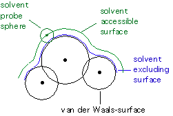
While calculation of the cavitation energy Gcav uses the surface
defined by the van der Waals-spheres, the solvent accessible surface is used
to calculate the dispersion-repulsion contribution Gdr to the solution
free energy. The latter differs from the former through additional consideration
of the (idealized) solvent radius. The electrostatic contribution to the
free energy in solution Ges uses an approximate version of the solvent
excluding surface constructed through scaling all radii by a constant factor
(e.g. 1.2 for water) and then adding some more spheres not centered on atoms
in order to arrive at a somewhat smoother surface.
Localization and calculation of the surface charges is approached through
systematic division of the spherical surface in small regions (tesserae)
of known area and calculation of one point charge per surface element.
The implementation of the PCM/UAHF model in Gaussian 98 can be invoked
using the SCRF keyword in combination with PCM-specific
modifiers. The solvent can be specified using the Solvent=
modifier to the SCRF keyword, acceptable solvent names being
Water, DMSO, NitroMethane, Methanol, Ethanol, Acetone, DiChloroEthane,
DiChloroMethane, TetraHydroFuran, Aniline, ChloroBenzene, Chloroform, Ether, Toluene, Benzene,
CarbonTetrachloride, Cyclohexane, Heptane, and
Acetonitrile. Additional options can be specified at the
end of the input file and read in using the Read
modifier of the SCRF keyword. The PCM solvation model is available for calculating
energies and gradients at the Hartree-Fock and DFT levels. The output generated
during PCM calculations can be dramatically extended using the DUMP
option.
The following sample input illustrates the use of the corresponding keywords
in the context of a single point calculation (without geometry optimization)
on the aqueous solvation free energy of ethanol in its Cs symmetric
conformation:
#P B3LYP/6-31G(d) scf=tight int=finegrid SCRF=(PCM,Read,Solvent=Water)

pcm/b3lyp/6-31G(d) sp ethanol in water (Cs)

0 1
O1
C2  1  r2
C3  2  r3  1  a3
H4  3  r4  2  a4  1  180.0
H5  3  r5  2  a5  4  d5
H6  3  r5  2  a5  4  -d5
H7  2  r7  3  a7  1  d7
H8  2  r7  3  a7  1  -d7
H9  1  r9  2  a9  3  180.0

r2=1.42492915
r3=1.51965095
r4=1.09569807
r5=1.09496362
r7=1.10264669
r9=0.96904984
a3=107.81130783
a4=110.63999342
a5=110.37205263
a7=109.90077195
a9=107.87777748
d5=-120.23659087
d7=-121.12750852

DUMP
|  |
The additional output caused by the PCM solvation model is
produced by link 502 responsible for the SCF calculation:
 ------------------------------------------------------------------------------
 Solvent: WATER
 Model  : PCM/UAHF, Icomp = 4
 Version: MATRIX INVERSION
 Cavity : PENTAKISDODECAHEDRA with  60 initial tesserae
 ------------------------------------------------------------------------------
 Nord Group  Hybr  Charge Alpha Radius            Bonded to
   1   OH    sp3   0.00   1.20  1.590     C2  [s]
   2   CH2   sp3   0.00   1.20  1.860     O1  [s]  C3  [s]
   3   CH3   sp3   0.00   1.20  1.950     C2  [s]
 ------------------------------------------------------------------------------

 ------------------------------------------------------
             Dielectric Const  =   78.39000
             High.Fr.D.Const   =    1.77600
             d(Diel.Const.)/dT =   -0.35620
             Molar Volume      =   18.07000
             Therm.Exp.Coeff.  =    0.00026
             Radius            =    1.38500
             Absolute temper.  =  298.00000
             Number of spheres =   3
             OMEGA             =   40.00000
             RET               =    0.20000
             FRO               =    0.70000
             Accuracy          =    0.1D-05
 ------------------------------------------------------
The first four lines repeat settings specific for water or
default settings for the PCM model in general. The solute cavity
is constructed from vdW-spheres represented through regular
pentakisdodecahedra, dividing each sphere's surface in 60 elements
of equal size.
The following four lines list the results of the UAHF analysis,
identifying only three (united atom) centers. For each
center the assumed hybridization is listed together with
its formal charge, the final radius, and the solvent-specific
scaling parameter Alpha. The latter usually defaults to
1.2, but can be specified directly using the option
ALPHA=x.x
The final part of the output lists solvent-specific parameters
such as the dielectric constant and the effective solvent radius,
together with some more default PCM settings such as the
number of initial spheres and the current values of parameters
OMEGA, RET, and FRO. These latter three parameters govern
the process of adding more spheres (not located at atomic
positions) in order to smooth the surface. New values for OMEGA
can be set using the option:
OMEGA=n.n
meaningful values ranging from 40.0 to 90.0 (higher values giving
less added spheres). New values for FRO can be specified with:
FRO=m.m
meaningful values ranging from 0.7 to 0.2 (smaller values giving
less added spheres). RET specifies the minimum radius of added new
spheres and new values can be specified with:
RET=l.l
increasing values giving less added spheres and very large values
avoid additional spheres completely.
The PCM algorithm then first runs through a gas phase energy calculation
in order to obtain a reference point for the subsequent solvation free
energy calculation. After completion of the gas phase SCF cycle, details
of the iterative process of cavity generation are listed:
 ------------------------------------------------------
 ----------  CAVITY for ELECTROSTATIC term  -----------
 ------------------------------------------------------
 -------  The SOLUTE is enclosed in ONE CAVITY  -------
          Total N.of Tesserae   =  132
           Surface Area (Ang**2) =   97.71529
           Volume       (Ang**3) =   84.60281
------------------------------------------------------
 Original Sphere   On Atom   Re0   Alpha      Surface
         1            O1     1.590  1.200      24.08112
         2            C2     1.860  1.200      27.26919
         3            C3     1.950  1.200      46.36498
 ------------------------------------------------------
 ------------------------------------------------------------------------------
     AT CONVERGENCE
  132 Tesserae over a maximum of 1500
  Surface Area (Ang**2) =   97.71529
  Volume       (Ang**3) =   84.60281
 Escaped Charge= 0.13334
 Error on NUCLEAR pol.charges = 0.21898 Error on ELECTR. pol.charges =-0.33812
 ------------------------------------------------------------------------------
 ------------------------------------------------------------------------------
    dG(solv)/dEps          (kcal/mol) =   0.00000
 ------------------------------------------------------
 IN VACUO Dipole moment (Debye):
   X=  0.0176  Y=  1.5625  Z=  0.0000  Tot=  1.5626
 IN SOLUTION Dipole moment (Debye):
   X=  0.1053  Y=  1.9429  Z= -0.0019  Tot=  1.9457
 ------------------------------------------------------
 Tessera     X         Y         Z        QTot      QSN       QSE
    1     2.84136   0.54870   3.42913   0.00354  -0.17977   0.18331
    .
    .
    .

  132    -2.70116  -2.26783  -4.13447  -0.00393  -0.25391   0.24997
In this (well behaved) case there is no need for additional spheres.
The overall surface is represented by 132 surface elements ("Tesserae").
The molecular volume as defined through the current surface does not
contain all the electron density of the system due to the long (in fact:
never ending) tails of the electronic wavefunction, giving rise some
"Escaped Charge". At the center of each surface element sits one surface
charge "QTot" containing one component from the nuclear charges of the
solute and one from the electronic charges of the solute.
The results obtained during solution of the electronic Schroedinger
equation (including the additional effects of the reaction field) are
then given as:
 SCF Done:  E(RB+HF-LYP) =  -155.041616090     A.U. after   10 cycles
             Convg  =    0.1222D-08             -V/T =  2.0093
             S**2   =   0.0000
 KE= 1.536131750668D+02 PE=-5.252140797608D+02 EE= 1.349508863800D+02
 ------------------------------------------------------
 -------------- VARIATIONAL  PCM  RESULTS -------------
 ------------------------------------------------------
    <Psi(0)| H |Psi(0)>        (a.u.) =   -155.033805
    <Psi(0)|H+V(0)/2|Psi(0)>   (a.u.) =   -155.040760
    <Psi(0)|H+V(f)/2|Psi(0)>   (a.u.) =   -155.041609
    <Psi(f)| H |Psi(f)>        (a.u.) =   -155.032883
    <Psi(f)|H+V(f)/2|Psi(f)>   (a.u.) =   -155.041616
    Total free energy in sol.
    (with non electrost.terms) (a.u.) =   -155.041162
 ------------------------------------------------------
    (Unpol.Solute)-Solvent (kcal/mol) =     -4.36
    (Polar.Solute)-Solvent (kcal/mol) =     -5.48
    Solute Polarization    (kcal/mol) =      0.58
    Total Electrostatic    (kcal/mol) =     -4.90
 ------------------------------------------------------
    Cavitation energy      (kcal/mol) =      8.92
    Dispersion energy      (kcal/mol) =    -11.39
    Repulsion energy       (kcal/mol) =      2.75
    Total non electr.      (kcal/mol) =      0.29
 ------------------------------------------------------
    DeltaG (solv)          (kcal/mol) =     -4.62
 ------------------------------------------------------
What is listed here as:
<Psi(0)| H |Psi(0)> (a.u.) = -155.033805
is the unperturbed gas phase SCF solution used as the reference
for all subsequent steps. The following energy described as:
<Psi(0)|H+V(0)/2|Psi(0)> (a.u.) = -155.040760
includes the interaction of the unpolarized solute with the
unpolarized solvent. Comparison with the gas phase reference energy
yields the corresponding interaction energy:
(Unpol.Solute)-Solvent (kcal/mol) = -4.36
After reporting the total energy corresponding to the interaction
of the unpolarized solute with the polarized solvent, the next
important information is that on the total energy of the polarized
solute:
<Psi(f)| H |Psi(f)> (a.u.) = -155.032883
The energy difference to the umpolarized gas phase total energy is
listed as:
Solute Polarization (kcal/mol) = 0.58
and should always be positive. The fully interacting
system of polarized solvent with polarized solute gives rise to
total energy:
<Psi(f)|H+V(f)/2|Psi(f)> (a.u.) = -155.041616
and the corresponding electrostatic interaction energy is listed as:
Total Electrostatic (kcal/mol) = -4.90
The non-electrostatic parts of the solvation free energy are given together
in one block terminated by the sum of the cavitation and the dispersion-repulsion
energies:
Total non electr. (kcal/mol) = 0.29
The sum of the electrostatic and non-electrostatic contributions gives the overall
free energy of solvation:
DeltaG (solv) (kcal/mol) = -4.62
It should be recognized, however, that the solvation free energy calculated here
refers to a motionless system in the gas phase at 0 Kelvin. In order to arrive at
thermochemically meaningful free energies at finite temperatures these solvation
free energies have to be augmented with a standard treatment of gas phase
thermochemistry. For the calculation of the solvation free energy itself as the difference
in gas and solution free energies this is often neglected and the value produced by
PCM is used directly in comparison to experimental values. For ethanol, the experimental
free energy of solvation has been measured as -5.0 kcal/mol. Compared to this value the
PCM prediction of -4.6 kcal/mol can be considered to be rather accurate.
When calculating solvation free energies as the difference of gas phase and solution phase
free energies attention must be paid to the definition of the respective standard states.
In case both the gas and solution phase concentrations are given in molar values (mol/l),
gas and solution phase data can be compared directly. Gas phase values refer, however,
often to a partial pressure of 1 atm. Assuming ideal gas behaviour, this corresponds to
1/24.46 mol/l at 298.15K.
An improved prediction of solvation free energies should also cover the effects of
structural relaxation in solution. Geometry optimizations using the PCM model are
possible, but much more time consuming than gas phase optimizations. This is not only
due to higher CPU times for each of the energy and gradient calculations, but also
due to a much slower convergence of the optimization process and frequent oscillations.
Two options that are helpful in alleviating some of the convergence problems are TSNUM
and TSARE:
TSNUM specifies the number of surface elements (tesserea)
for each sphere. The PCM algorithm selects regular polyhedra whose number of
surface elements are as close as possible to TSNUM. Aside from the default value
of 60, some larger values such as 64, 80, or 100 may be helpful in reducing the
oscillatory behaviour in some geometry optimizations.
TSARE specifies the area of the surface elements in units
of (Angstroms)2. Meaningful values range from 0.4 to 0.2, smaller values leading
to a larger number of surface elements. Setting the size of the surface elements to
a particular value leads to surface elements of equal size, regardless of the radius
of the sphere (this is not the case when TSNUM settings are changed).
In both cases, however, the total energies depend on the actual choice of surface
elements and a comparison of results for different systems or different conformers is
only meaningful with the same choice of options. For the ethanol example used here
the geometry optimization does not converge within 23 steps using the default settings,
but can be brought to convergence within 7 steps using TSARE=0.3, yielding a final
total energy in solution of -155.043097702 au. Compared to a PCM single point calculation
using the gas phase geometry (with total energy of -155.041371 au) this implies a
structural relaxation energy of -1.1 kcal/mol and thus an "improved" prediction of
the solvation free energy of -5.7 kcal/mol.
One problem when applying the current implementation of the PCM/UAHF model to reaction
pathways in solution is a direct consequence of using hybridization and connectivity data
for the derivation of the vdW radii. As both hybridization and connectivity are not
going to change smoothly but suddenly from one point to the next along a reaction pathway,
the UAHF approach is bound to produce sudden breaks in the free energy of solvation
profile. These problems can, in principle, be circumvented by smoothly scaling
from one set of radii to another, or by avoiding the UAHF approach altogether
and choosing radii that don't depend on connectivity. One common choice for the
latter case are Pauling radii available with the option
RADII=Pauling.
More recent versions of Gaussian contain a strongly revised version of the PCM
model, in particular with respect to the definition of the solute cavity. This has also brought
some changes to the list of acceptable keywords. The following example illustrates the keywords
PCMDOC (formerly DUMP), RADII, and
SCFVAC.
#P B3LYP/6-31G(d) scf=tight int=finegrid SCRF=(PCM,Read,Solvent=Water)

pcm/b3lyp/6-31G(d) sp ethanol in water (Cs)

0 1
O1
C2  1  r2
C3  2  r3  1  a3
H4  3  r4  2  a4  1  180.0
H5  3  r5  2  a5  4  d5
H6  3  r5  2  a5  4  -d5
H7  2  r7  3  a7  1  d7
H8  2  r7  3  a7  1  -d7
H9  1  r9  2  a9  3  180.0

r2=1.42492915
r3=1.51965095
r4=1.09569807
r5=1.09496362
r7=1.10264669
r9=0.96904984
a3=107.81130783
a4=110.63999342
a5=110.37205263
a7=109.90077195
a9=107.87777748
d5=-120.23659087
d7=-121.12750852

PCMDOC
RADII=UAHF
SCFVAC
| |
The last of the keywords forces the program to first calculate the unperturbed gas phase wavefunction
and afterwards the one in solution. While this is the default in earlier versions of Gaussian,
the current default is to only perform the solution calculation. A second major change concerns the
choice of default radii. While UAHF radii have been the default choice in earlier versions of
Gaussian, the newer version use United Atom Topological Model (UA0) radii by default. This
is not necessarily the best choice and some experimentation is required as to which electronic structure
method fits which type of radii best. United Atom radii optimized to fit density functional methods
particularly well have been optimized for the PBE/6-31G(d) level of theory and can be used with
RADII=UAKS. The TSARE keyword has retained its
previous meaning, but defaults now to a value of 0.2 (Angstroms)2.
last changes: 01.04.2008, AS
questions & comments to: axel.schulz@uni-rostock.de