In the region of correct negative curvature, that is, in the vicinity of the actual transition state, one can use a local searching method to optimize the transition state structure. In order to work at all, it is therefore mandatory to provide a reasonable starting structure, which might either be obtained by guessing well or by a series of constrained optimizations (relaxed potential energy scans). Taking the isomerization of HCN to CNH again as an example, we could take the structure of highest energy along the hydrogen migration pathway and search from there using a local gradient method:

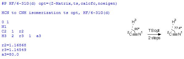
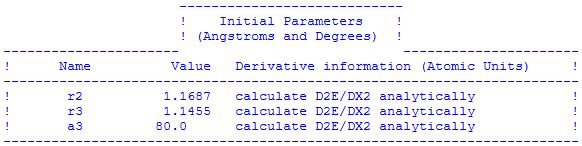
The transition state optimization (ts) is specified here in terms of an internal coordinate system (Z-Matrix) and is based on a Hessian matrix calculated at the first point of the optimization process (calcfc). As more than one negative eigenvalue might appear in the Hessian matrix during the optimization procedure, we turn off checking the eigenvalues with noeigen. Explicit calculation of the Hessian matrix at the beginning of the optimization procedure is expensive, but necessary in transition state optimizations. That the second derivatives are actually calculated for all structural parameters can be seen at the beginning of the output file:

After each geometry optimization step the output file contains the current Hessian matrix, its eigenvalues, as well as the corresponding eigenvector:

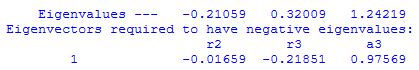
In this very simple case containing only three structural variables, there is indeed only one large and negative eigenvalue, the corresponding eigenvector being dominated by the angle a3. Transition state searches will usually only work if there is at least ONE negative eigenvalue. Multiple negative eigenvalues will not be a problem as long as one of these is significantly larger than all the others. The optimization algorithm follows the most negative (largest) eigenvalue in the optimization process.

With the derivative information in hand, the Berny algorithm steps into the supposedly correct direction uphill, at the same time lowering the energy gradient. For the new structure, a new Hessian is obtained using the previous Hessian and gradient information of the last points. This updating scheme is usually sufficient to lead to a successful transition state optimization within a small number of optimization cycles. If, however, the optimization is not successful after 10-15 optimization cycles while the structure of the system has changed considerably, a completely new Hessian should be generated by restarting the optimization with calcfc.

In the current case, the optimization takes only two steps until the default convergence criteria are fulfilled and the transition state is found with a bond angle of A(H-C-N)=77.4424 degrees, bond distances R(C-N)=116.92 pm and R(H-C)=115.46 pm, and an HF/6-31G(d) total energy of -92.7919533 Hartree. Relative to the respective HCN ground state with R(C-N)=113.25 pm, R(H-C)=105.90 pm, and a total energy of -92.8751975 Hartree, this represents an activation energy of +218.6 kJ/mol.

This system can also be used to demonstrate the importance of a good starting point for the transition state search. If the search is initiated from a bond angle of a3=90.0 instead of a3=80.0, the starting point is located further away from the actual transition state at a3=77.4424 degrees. Using this starting point, the transition state is located after four optimization cycles. Choosing larger initial bond angles of 100.0 or 110.0 degrees leads to even longer transition state searches of five or six steps.

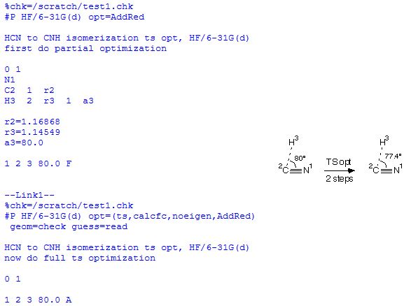
In many cases an approximate transition state structure (and thus a good starting point for the transition state optimization) cannot be generated using the scanning strategies. This may either be too costly or due to the fact that the reaction path is described by more than one structural variable. In this situation it is desirable to generate a starting structure for the transition state optimization using a constrained optimization. The following example shows how the hydrogen migration transition state in HCN can be located following this strategy.

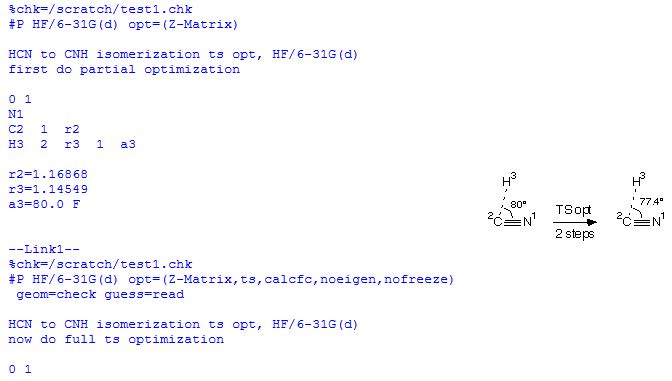
The first part of this compound job will perform a partial geometry optimization in the Z-Matrix coordinates given in the input file, freezing the bond angle a3 to a value of 80.0 degrees. In the second job step the preoptimized geometry is retrieved from the checkpoint file and the constrained bond angle is freed up using the nofreeze option of the opt keyword. This is reflected in the output file at the point of geometry retrieval:

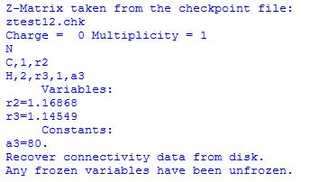
Should there be more than one frozen variable then all of these constraints will be lifted at this point. The other keywords specify a transition state optimization after initial calculation of the Hessian. The transition state located in this fashion is identical to the one found before. The same sequence of steps can be performed in redundant internals using the following compound job: