Vibrational Frequencies - Technical Considerations
Selecting a Structure
One of the first conditions that must be satisfied in order to perform an accurate calculation of vibrational frequencies is that the underlying molecular structure represents a stationary point, that is, all first derivatives of the energy with respect to nuclear coordinates must be essentially zero. Using the vibrational frequency spectrum for the dihydrogen molecule (H-H) as an example, one can show that smalldeviations from the equilibrium structure can quickly lead to large errors in the calculated vibrational frequencies. The experimentally measured fundamental vibrational mode is located at 4160 cm-1. Expanding the vibrational frequencies in a series containing harmonic and anharmonic terms, the corresponding (experimental) harmonic frequency is 4401 cm-1. The following values are obtained at the HF/6-31G level of theory using structures optimized to different accuracy:
All six structures summarized in the table above have rather similar total energies, the energy difference between the most favorable structure (last entry) and the least favorable structure (first entry) being less than 1 kJ/mol. The structural differences for these two structures amount to less than 1% (only 0.5 pm) in the H-H bond distance, giving rise to a residual gradient for the least favorable structure of 3.86*10-3au. Compared to these differences in structure, energy and gradient, the changes in the calculated vibrational frequencies are much more pronounced. For a linear molecule with two atoms we expect only one real vibrational mode in addition to five near-zero modes describing translational and rotational motion. This latter expectation is not fullfilled for the first five entries in the table as in particular the two rotational modes are far from zero. The H-H stretching mode also suffers from the residual gradient, showing variations of almost 80 cm-1. That the predicted harmonic frequency for the H-H streching mode appears to converge to a value further away from the experimentally measured one with decreasing residual gradient is primarily due to deficiencies of both the Hartree-Fock model as well as the small basis set (see below), but not a consequence of insufficient geometry optimization.
Similar results are obtained with other theoretical methods whose second derivatives cannot be calculated analytically and thus require a numerical algorithm. This is the case for the semiempirical AM1 method:
We observe that the AM1 value converges to 4342 cm-1 with increasing accuracy of the geometry optimization. Again we note a large variation in predicted vibrational frequencies with an increasing residual gradient. In contrast to the HF results discussed before the five translational and rotational modes cannot be converged to very small values now. This is a consequence of additional problems of numerical vibrational frequency calculations (see below).
Selecting an Algorithm
Calculation of the force constant matrix (Hessian) can be performed with two different algorithms:
1) Using an analytical algorithm. The keyword for this option in Gaussian is
freq=Analytic
and it is the default for those theoretical methods, for which analytical second derivatives are available. The latter include Hartree-Fock theory (HF), all density functional methods (DFT), as well as MP2. Analytical calculation of the force constants is significantly faster and also more accurate than the alternative approach:
2) Using a numerical method. The keyword for this option in Gaussian is
freq=Numerical
and it is the default for methods for which analytical second derivatives are not available in Gaussian such as all semiempirical methods. For this option, the algorithm involves double displacements of all centers in all three cartesian coordinates. The step size used in this procedure can be specified with
freq=(Numerical,Step=N)
N being the size of the step in units of 0.0001 Angstroms. The default value for N is 100 in semiempirical calclations. Smaller values require a somewhat tighter convergence criterion for the energy calculations as the unperturbed and perturbed structures are structurally and energetically rather similar. This can be specified with
scf=(Conver=n)
which sets the convergence criterion in energy calculations to 10-n Hartree on two successive SCF iterations. The default for semiempirical calculations such as AM1 is n=6, but values of n=7 or 8 are more appropriate once the step size in numerical second derivative calculations is less than N=50. Using these options, the vibrational frequency calculation for H2 (AM1 level, H-H distance = 67.659 pm) can be modified as follows (the principal stretching vibration is again shown in bold):
The last entry in this table marks the limits of numerical accuracy that can be achieved with this approach.
Differentiating Ground and Transiton States
Pushing the limits of vibrational frequency calculations is sometimes necessary in order to achieve unequivocal characterization of minima and transition states on the potential energy surface. While minima are expected to show 6 very low frequencies in their vibrational frequency spectrum (3 for translational and 3 for rotational motions in a non-linear system) one large negative and 6 very small frequencies are expected for a transition state. The vibrational spectra calculated for methanol (CH3OH) will be used as an example. For this system one would expect 3*6 - 6 = 12 true vibrational modes. The lowest seven vibrational modes are shown in the following tables, first for the staggered and then for the eclipsed conformer (HF/6-31G(d) results):
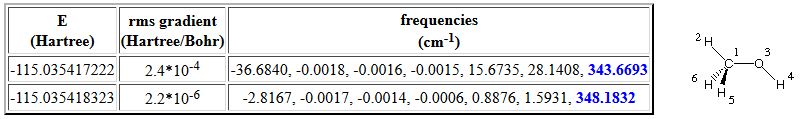
This first conformer shows one larger imaginary frequency (-37 cm-1), then three close-to-zero values, two small positive vibrations of 16 and 28 cm-1 and finally one larger vibrational mode at 344 cm-1. Is this a transition state or a local minimum? Even though we are clearly not having one large imaginary frequency in combination with sixe close-to-zero values as expected for a transition state, the six lowest vibrational frequencies are not all that close to zero. The second entry in the table above shows that a clear case can be made for a local minimum after reoptimization to a higher convergence criterion.
Geometry optimization of the eclipsed conformer of methanol using loose convergence criteria leads to a first structure whose vibrational frequency spectrum contains a number of imaginary vibrational frequencies (first entry in the following table):
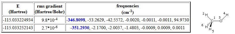
Reoptimization of the same structure with tighter convergence criteria leads to a much clearer result and we can recognize that the lowest true vibrational mode of the staggered conformer at 348 cm-1 turns into an imaginary mode of 351 cm-1 in the eclipsed structure. Both modes describe rotational motion around the central C-O bond.
In contrast to the analytical algorithm, failed numerical frequency calculations can be restarted with
freq=(Numerical,Restart)
Scaling Vibrational Frequencies
A final point concerns the accuracy obtained in vibrational frequency calculations as a function of the theoretical method used. In many cases, the experimentally measured values will differ significantly from those calculated theoretically. One source of discrepancy is that experimental values are often measured in solution while calculated values refer to the gas phase. A second source of error is the assumption of the harmonic approximation. There is, however, also a method-dependent difference between calculated and experimentally measured harmonic vibrational frequencies in the gas phase. For more economical methods such as HF or AM1, the deviations typically range around 10%. In order to account for this systematic deviation, all vibrational frequencies can be scaled (=multiplied with the same value) down to fit the experimental harmonic frequencies. Radom et al. have published a list of recommended scale factors for frequently used theoretical methods in J. Phys. Chem.1996, 100, 16502. A small selection is:
It is clear from these results that semiempirical methods such as AM1 and PM3 will, even after scaling, not be particularly reliable in predicting vibrational spectra. Rather good results can be obtained either from highly correlated, expensive methods such as QCISD, or from hybrid density functional calculations such as B3LYP.
Further Reading
A detailed discussion of further aspects of vibrational frequency calculations in Gaussian has been published by Joseph W. Ochterski (Gaussian Inc.) and can be found on the Gaussian home page: Vibrational Analysis in Gaussian.